Banana random number generator part 2: chi-squared, ent, timers, interrupts

Read the first part here.

In the previous post we addressed the basic concepts of the generator, leaving open the question of the bad chi-square. Before delving into the reasons for the bad result, it is necessary to understand what this value is and how randomness is “extracted” from a radiation event.

Let’s start by understanding what the chi-square (also referred to as ) is and how it works. This is a value used in statistics to test the fit of a set of values to a theoretically predicted distribution. Let’s address the traditional use in statistics first, then we’ll turn our gaze to the use of for this application.

Given a data set, we call frequency the number of times a given data item occurs, and degrees of freedom the number of possible values minus one. Why minus one? This operation, which at first glance may seem quite strange, is actually very logical. Suppose we want to analyze the tossing of a coin. We have two possible outcomes: heads and tails. If we think about it, however, the percentage of times it comes up heads is directly determined by the percentage of times it comes up tails. If we consider an event with three possible outcomes, the percentage of the third outcome is directly determined by the other two. In this sense, we speak of degrees of freedom. 

The chi-square formula is:

   

where is the observed frequency and is the theoretically expected frequency.

Let us take as an example the classical roll of a six-sided die. The throw of the die can result in six possible outcomes, this gives us 5 degrees of freedom. Imagine throwing the dice 1000 times, we want to verify what in statistics is called hypothesis zero, or verify that, within a certain probability, our results are truly random.  These are the data we get from our experiment:

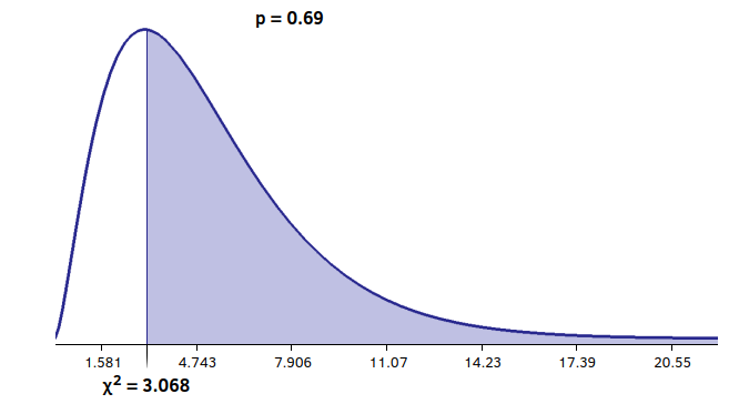
Adding up the individual contributions, we get the chi-square value of our experiment: 3,068. Now what? Let’s take a second to think about the data and our formula, keeping in mind that we are trying to measure, in this case, how closely our data adhere to a uniform distribution. If everything were perfect (in a hypothetical dimension where this can happen), we would have the observed frequencies equal to the theoretical frequencies , so our denominator . Consequently . However, we know that perfection does not belong to our world, otherwise we would not even need statistics. In other words, it is extremely unlikely that our data exactly reflects the theoretical distribution, a value of chi square too close to zero should make us suspicious.

On the other hand, the further we move away from the theoretical distribution, the more the numerator grows, with the same denominator. Which causes the chi-square value to grow. This for the normal use of chi-square is very good news, it means being able to reject the null hypothesis, and therefore knowing that you are working with data that are not just the result of chance, but have some meaning. For our application, however, this would mean bad news: it would mean that our data is not uniformly distributed.

This means that, for our application, we’ll have to look for a middle ground. Okay, but numerically? The acceptable chi-square value varies based on the degrees of freedom of the system. This is where the hard part begins, made up of unfriendly integrals and equations that cannot be solved algebraically [2]. Fortunately someone has already done the work for us, arranging the results in tables conveniently available on the internet.

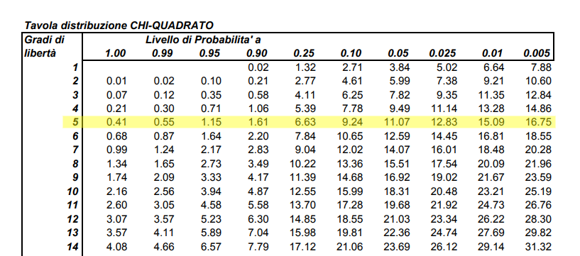
The rows of the table represent the degrees of freedom of the system, in our case of the die there are 5. The columns represent the probability levels that the calculated value is greater than the tabulated value. There are also tables that indicate the probability that the calculated value is less, these are called left tail tables, while the one shown above is a right tail table. This is because in one case the right side of the graph is considered, and in the other the left side. In our case we have , which is between 90% and 25% of the cases. This is enough to say that there is no excessive variation from behavior that we can classify as random. [3]

Going back to bananas, let’s take 90% and 10% as reference percentages. Unfortunately I was not able to find tables for 255 degrees of freedom, but fortunately the author of ent provides a tool to calculate the values for each probability [2].
For 255 degrees of freedom () we have the values: and . From ent’s tests on the values recorded by the generator, we had obtained a value of 498.15, definitely out of the range of acceptability. The probability percentage returned by ent was .
.
Ent, using the -c option returns the frequency of each byte, which is shown below, omitting the insignificant bytes (4 to 253):

valerio@valerio ~/tests $ ent logbinario.txt -c
Value Char Occurrences Fraction
  0              739   0.004077
  1              402   0.002218
  2             1033   0.005699
  3              674   0.003718
...              ...      ...       
254   �         722   0.003983
255   �         691   0.003812

Total:        181256   1.000000

Entropy = 7.997995 bits per byte.

Optimum compression would reduce the size
of this 181256 byte file by 0 percent.

Chi square distribution for 181256 samples is 498.15, and randomly
would exceed this value less than 0.01 percent of the times.

Arithmetic mean value of data bytes is 127.4942 (127.5 = random).
Monte Carlo value for Pi is 3.138799695 (error 0.09 percent).
Serial correlation coefficient is 0.005408 (totally uncorrelated = 0.0).

You immediately notice that byte 1 has significantly fewer counts than the others, and that byte 2 has many more. At a closer look, the counts that seem to be “missing” 1, are assigned to 2. This is definitely our problem.

After some fruitless testing, I decided to split the even position bytes from the odd position bytes. This is because for every 16-bit number (2 bytes) generated, two bytes are created, one of even position and one of odd position. I basically divided the file into Most Significant Byte and Least Significant Byte. These are the results:

valerio@valerio ~/tests $ ent logbinariomsb.txt -c
Value Char Occurrences Fraction
  0              358   0.003950
  1              393   0.004336
  2              347   0.003829
  3              333   0.003674
...              ...     ...
254   �          374   0.004127
255   �          330   0.003641

Total:         90628   1.000000
...
Chi square distribution for 90628 samples is 240.88, and randomly would exceed this value 72.82 percent of the times.
...

valerio@valerio ~/tests $ ent logbinariolsb.txt -c
Value Char Occurrences Fraction
  0              381   0.004204
  1                9   0.000099
  2              686   0.007569
  3              341   0.003763
...              ...     ...
254   �         348   0.003840
255   �         361   0.003983

Total:         90628   1.000000
...
Chi square distribution for 90628 samples is 891.23, and randomly would exceed this value less than 0.01 percent of the times.
...

The MSB group does not report any significant problems, while the LSB group is where the problem lies.

To understand where this problem originates, we must first understand how the numbers are generated internally. The geiger tube, via an interface circuit, sends a signal on pin 2 (PB2/INT0) of the arduino when it is hit by radiation. Pin 2 is configured to generate an interrupt when it receives a rising edge: attachInterrupt(digitalPinToInterrupt(2), randomCore, RISING);. The interrupt will call the randomCore() function, which is defined as follows:

void randomCore() {
  Serial.println((unsigned int)(( micros() >> 2 ) & 0xFFFF));
  return;
}

The function, when called, in turn calls the arduino’s micros() function. This function returns a 32-bit number that represents the number of microseconds that have elapsed since the system was turned on. Being a 32-bit unsigned number, it will overflow after 4294.96 seconds, or every 70 minutes or so. Since the speed of the microcontroller is insufficient to obtain a more accurate update, micros() updates in jumps of 4 microseconds, always keeping the two least significant bits at zero.

For this reason, we perform a shift of the value returned by micros() by two bits to the right. In this way we get a value of 30 bits. If we also used the least significant bits, we would get progressive numbers until the next timer overflow. Each number would definitely be greater than the previous and definitely less than the next, over the 70 minutes it takes for the overflow to occur. This is definitely not random. 

Let’s therefore preserve only the first 16 bytes of the micros(). This value will have overflows every 262144 microseconds, making it extremely unlikely that the above situation will occur. (The geiger counter background records about 30 pulses per minute).

Thus, the problematic value is as follows, where the MSB is irrelevant:

16       8         0
XXXX XXXX 0000 0001 

It caught my attention that this value occurs every 4*2^8 = 1024 microseconds, or about 1 millisecond, and is the next value after the one that generates an interrupt overflow. My attention then shifted to the code of the millis() function of the arduino core [4] [5].

The core’s millis() function works by setting the TIMER0 prescaler to 64, which for an 8-bit timer with a 16MHz clock results in a timer overflow every 1.024 milliseconds. The timer overflow generates an interrupt, with vector TIMER0_OVF. If the geiger tube pulse arrives at the same time as the TIMER0 overflow, we will have two competing interrupts: TIMER0_OVF and INT0. This situation is handled by the microcontroller with an interrupt priority system, whose priority order is indicated in the datasheet:

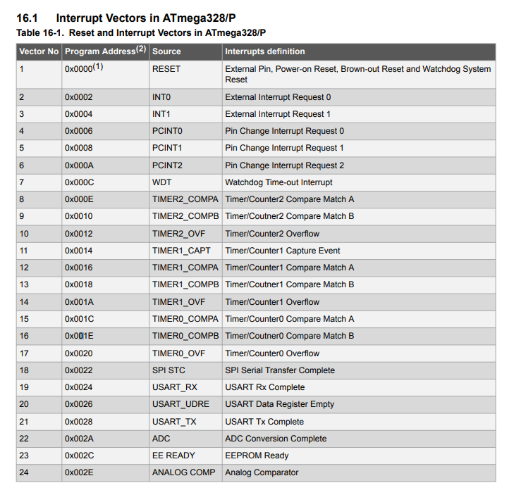
The TIMER0 overflow has much lower priority than the external interrupt, so my guess is as follows:

1. Case 1: The INT0 interrupt arrives at the same time as the TIMER0_OVF interrupt. Since it has a higher priority, the external interrupt is executed first at the expense of millis(), affecting the accuracy of the function but without producing visible effects on the generated numbers;
2. Case 2: the INT0 interrupt arrives at the next clock cycle than the TIMER0_OVF interrupt. Since one clock cycle has already elapsed, the TIMER0_OVF interrupt will already be executing. When execution is finished, micros() will already be at value 2, so the generated number will be registered with value 2. 

It is possible that the use of serial also has an influence on this delay, but I have not investigated this further. The solution to this problem will be exposed in a future post, and it implies the use of TIMER1 for number generation, instead of the micros() function of Arduino.

I want to thank Mauro Mombelli and the StackExchange cryptography community for their valuable help [7] [8].

Notes, sources and links:
[1] BRNG: generare numeri casuali a partire dalle banane
[2] Fourmilab – chi-squared calculator
[3] How to evaluate chi-squared results
[4] Millis in wiring.c su github
[5] µC eXperiment blog – Examination of the Arduino millis() Function
[6] Datasheet dell’ATMega328/P
[7] StackExchange Cryptography – Random number generator issue
[8] StackExchange Cryptography – How to evaluate chi squared result?
[9] AVRBeginners – Timers

This work is licensed under a Creative Commons Attribution-NonCommercial-ShareAlike 4.0 International License.